ROC_PRC_visualizer
A web-based biostat app to visualize region of utility of an ROC or PRC given the pretest probability (prevalence).
Region of Utility – brief statement
In a diagnostic test, the usual measure of how "good" (i.e. discriminative) it is in general is based on certain features of the ROC curve such as its area under the curve or the closeness of its peak to the top left corner of the curve. However, a generally "good" test may not be applicable to all situations given certain disease prevalence and a need to achieve minimal positive predictive value (PPV) or negative predictive value (NPV). Therefore, I propose here another measurement titled the region of utility, referring to a limited estate within the square coordinate of the ROC or PRC curve defined by one’s desired thresholds for minimal sensitivity (i.e. recall), PPV (i.e. precision), and NPV. For a test to be useful, its curve must fall within this region of utility. Only then can one choose the best test threshold from within this region – i.e. the point on the ROC curve closest to the top left corner. We present a web-based interactive visual representation (https://reirisono.github.io/ROC_PRC_visualizer/visualizer.html as of 20211102) with its derivation explained below.
Supplementary Document: ROC curve interpretation 20191025 Reiri Sono
Receiver operating characteristic (ROC) curve plots Sensitivity over 1-Specificity, two variables independent of disease prevalence. These parameters are alternatively called true positive rate (TPR) over false positive rate (FPR), which can be confused with True Positive (TP) and False Positive (FP). This section goes over the interpretation of the Sensitivity over 1-Specificity (“Sens/Spec”) curve relative to changes in Positive Predictive Value (PPV) and Prevalence, then translates it to a hypothetical plot of TP over FP (“TP/FP curve”) dependent on Prevalence. It will discuss how each coordinate system can express region of utility, dictated by PPV, in order to indicate the practical limitation of choice of test threshold. It will visualize how the TP/FP curve spatially “contains” an axis-scaled version of the Sens/Spec curve. It will walk through the derivation of each key term on the Sens/Spec and TP/FP curve.
The rest of the document will refer to variables A, B, C, D according to this 2x2 predictor-outcome matrix derived from disease and healthy samples reflecting the disease prevalence:
|
Test \ Disease |
Disease (+) |
Disease (-) |
Subtotal |
|
Test (+) |
A |
B |
A+B |
|
Test (-) |
C |
D |
C+D |
|
Subtotal |
A+C |
B+D |
A+B+C+D=1, i.e. 100% |
<![if !msEquation]><![if !vml]>![]() <![endif]><![endif]>
<![endif]><![endif]>
<![if !msEquation]><![if !vml]>![]() <![endif]><![endif]>
<![endif]><![endif]>
<![if !msEquation]><![if !vml]>![]() <![endif]><![endif]>
<![endif]><![endif]>
<![if !msEquation]><![if !vml]>![]() <![endif]><![endif]>
<![endif]><![endif]>
Note that the equations
of Prevalence, Odds Ratio, and PPV apply only when the
diseased and healthy samples were taken proportionally to reflect the disease
prevalence.
Sensitivity and Specificity are both independent of prevalence. The graph below is an example of diagnostic test that returns a higher value, albeit with overlap, in the diseased population, hence (+) when the value is high. Using the 2nd diagram, each quadrant of the 2x2 matrix can be visually represented as these colored areas:
<![if !vml]>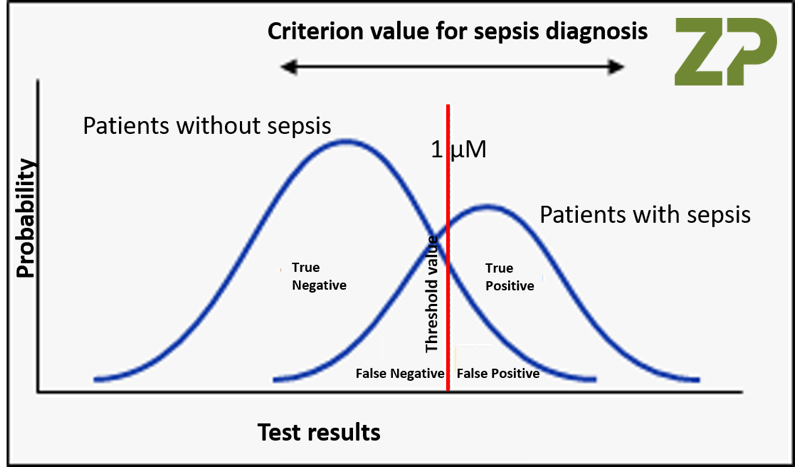 <![endif]><![if !vml]>
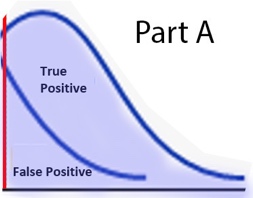 <![endif]><![if !vml]>
![]() <![endif]>
<![endif]>
<![if !vml]>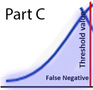 <![endif]> <![if !vml]>
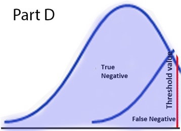 <![endif]>
Since Sensitivity and Specificity each is a ratio within the same bell curve, the sizes of the bell curves are factored out, i.e. do not affect sensitivity or specificity.
Sens/Spec curve: Y = Sensitivity, X = (1-Specificity)
Using a stricter threshold for test positivity is represented as sliding the vertical red bar to the right on the 2nd diagram. This alters the Sensitivity and 1-Specificity in the following way, explaining how a stricter threshold is represented as a coordinate along the bottom left of the curve B on the Sens/Spec curve.
|
|
Strict threshold (to the right on the double bell curves, if large value = (+) test so that diseased population more likely tests (+); to the left if otherwise) |
Lenient threshold (to the left on the double bell curves, if large value = (+) test so that diseased population more likely tests (+); to the right if otherwise) |
|
Sensitivity |
0 ≤ low |
high ≤ 1 |
|
1-Specificity |
0 ≤ low |
high ≤ 1 |
|
slope through origin = LR+ |
∞ ≥ high |
low ≥ 1 |
|
slope through (1,1) = LR- |
high ≤ 1 |
low ≥ 0 |
<![if !vml]>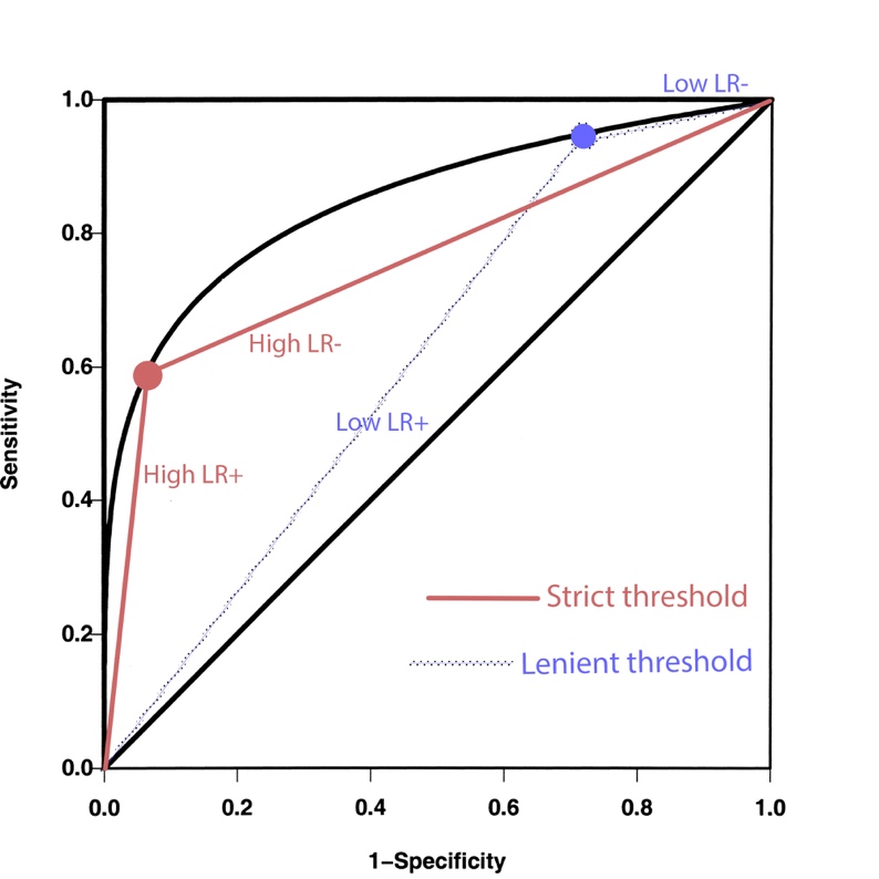 <![endif]>
FYI: The top left corner (X, Y) = (0, 1) represents the
perfectly discriminative test that all tests should aspire to; however, overlaps
in the result bell curves of disease (+) and (-) groups precludes reaching this
point. The diagonal line with slope = 1 represents a “no skill” test with no discriminative
power, i.e. where the bell-shaped histograms of the test results in the Disease
(+) & Disease (-) populations completely overlap, hence rendering an
identical values for <![if !msEquation]><![if !vml]>![]() <![endif]><![endif]> & <![if !msEquation]><![if !vml]>
<![endif]><![endif]> & <![if !msEquation]><![if !vml]>![]() <![endif]><![endif]> identical no matter where the red threshold
is.
<![endif]><![endif]> identical no matter where the red threshold
is.
Experiment: region of utility defined
by desired PPV & NPV and local Prevalence
Question: given a Prevalence and desired PPV
and NPV, what is the range of Sensitivity and Specificity
that a test can achieve? What are the tradeoffs?
Indication: This thought process is used to select the best
test for the purpose: only those with a curve that crosses or loops above the
required Sensitivity and Specificity coordinate can perform at
the desired PPV, NPV, and practical limitation of Prevalence.
PPV and NPV are inevitable
results of Sensitivity, Specificity, and Prevalence:
<![if !msEquation]><![if !vml]> <![endif]><![endif]>
<![if !msEquation]><![if !vml]> <![endif]><![endif]>
These transformations are useful in that they separate contributions to PPV or NPV into test-dependent (threshold-dependent to be exact), population-independent variables (Sensitivity, Specificity, LR+, LR-) vs. test-independent, population-dependent variable (Prevalence and Odds Ratio). Sliding along the test threshold:
|
|
Strict threshold |
Lenient threshold |
|
PPV |
high ≤ 1 |
low ≥ Prevalence |
|
NPV |
low ≥ 1-Prevalence |
high ≤ 1 |
Transforming this equation to answer the question: given a Prevalence and a minimum goal PPV and NPV, what range of the LR+ and LR- must be satisfied?
<![if !msEquation]><![if !vml]>![]() <![endif]><![endif]>
<![endif]><![endif]>
<![if !msEquation]><![if !vml]>![]() <![endif]><![endif]>
<![endif]><![endif]>
<![if !msEquation]><![if !vml]>![]() <![endif]><![endif]>
<![endif]><![endif]>
<![if !msEquation]><![if !vml]>![]() <![endif]><![endif]>
<![endif]><![endif]>
The equation shows that the slope through the origin, i.e. LR+,
must be at least as steep as the minimum goal PPV. In other words, the region
of utility (i.e. required range of Sensitivity and 1-Specificity for
a diagnostic test to be useful) resides on the top left corner triangle of the
ROC curve bound by the Y axis, the top edge (i.e. the Y=1 horizontal line), and
the line represented by <![if !msEquation]><![if !vml]>![]() <![endif]><![endif]>.
This condition dictates how strict the test threshold must be: a higher Prevalence
will raise OR, drop minimal required LR+, and thus open
up the region of utility; a lower Prevalence will raise minimal
required LR+ and thus narrow down the region. It makes
sense conceptually: when disease prevalence is high, a test with relatively
high false (+) rate (i.e. mediocre specificity) may still manage to predict (+)
disease with a (+) result at a satisfactory rate (i.e. satisfactory PPV).
<![endif]><![endif]>.
This condition dictates how strict the test threshold must be: a higher Prevalence
will raise OR, drop minimal required LR+, and thus open
up the region of utility; a lower Prevalence will raise minimal
required LR+ and thus narrow down the region. It makes
sense conceptually: when disease prevalence is high, a test with relatively
high false (+) rate (i.e. mediocre specificity) may still manage to predict (+)
disease with a (+) result at a satisfactory rate (i.e. satisfactory PPV).
For NPV, the watershed line defining the region of
utility is drawn from the top right corner, bounded by the Y axis, the top
edge, and <![if !msEquation]><![if !vml]>![]() <![endif]><![endif]>.
This condition dictates how lenient the test threshold must be: a higher Prevalence
raises OR, restricting the maximum allowed LR-, narrowing
down the region of utility; a low Prevalence raises maximum
allowed LR-, opening up the region. Together with the rule on
PPV, the region of utility is restricted from both the lenient
and strict ends of test threshold.
<![endif]><![endif]>.
This condition dictates how lenient the test threshold must be: a higher Prevalence
raises OR, restricting the maximum allowed LR-, narrowing
down the region of utility; a low Prevalence raises maximum
allowed LR-, opening up the region. Together with the rule on
PPV, the region of utility is restricted from both the lenient
and strict ends of test threshold.
<![if !vml]>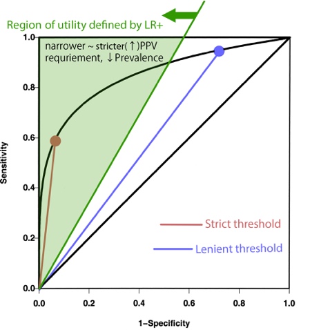 <![endif]><![if !vml]>
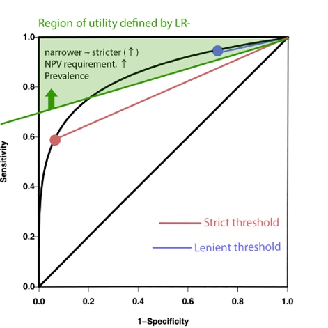 <![endif]><![if !vml]>
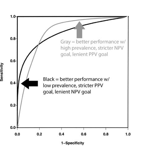 <![endif]>
Now that the region of utility is declared, it must be determined whether a diagnostic test can perform adequately within that region, and what threshold gives optimal performance. Any portion of its ROC curve that resides within the region of utility satisfies the LR+ and LR- slope requirements. Some test may have no portion in the region despite having a better performance characteristic overall. Within this portion, one must determine which point is closest to the top left corner, (X, Y) = (0, 1). The precise derivation depends on the exact shape of the ROC curve.
TP/FP and FN/TN curves
In the TP/FP version of ROC, the Y axis = A and X axis = B as
per the 2x2 matrix. Let us attempt to describe A as a function of B, Sensitivity,
Specificity, and Prevalence. First, we know that (A, B) and (C,
D) are each related by PPV = A/(A+B) and NPV = D/(C+D). Switching around to isolate A and C:
<![if !msEquation]><![if !vml]>![]() <![endif]><![endif]>
<![endif]><![endif]>
<![if !msEquation]><![if !vml]>![]() <![endif]><![endif]>
<![endif]><![endif]>
Substitute PPV and NPV with the equation from previous section:
<![if !msEquation]><![if !vml]> <![endif]><![endif]>
<![if !msEquation]><![if !vml]>![]() <![endif]><![endif]>Plugging
this “slope” term into the end of the above equation:
<![endif]><![endif]>Plugging
this “slope” term into the end of the above equation:
<![if !msEquation]><![if !vml]>![]() <![endif]><![endif]>
<![endif]><![endif]>
<![if !msEquation]><![if !vml]>![]() <![endif]><![endif]>
<![endif]><![endif]>
These forms are ready for experiments with tweaking the test threshold or disease prevalence one dimension at a time.
Experiment: tweak the LR terms
The likelihood ratios are completely dependent on the test
threshold and independent of disease prevalence. This term also happens to be
the slope that each connects (X,Y) = (0,0) or (1,1) and the specific coordinate
along the Sens/Spec ROC curve.
Suppose that the threshold is made the most lenient, such that all patients test (+) regardless of disease status. Then Sensitivity=1, Specificity=0, plotted @ the top right corner of this graph. At the same time, this condition renders the TP vs FP (i.e. A vs B) relation as:
<![if !msEquation]><![if !vml]>![]() <![endif]><![endif]>
<![endif]><![endif]>
Therefore, at the most lenient threshold, A becomes a
function of B and prevalence alone.
Any stricter threshold renders the LR+ term ≥ 1, as evidenced by how the slope steepens from line C to the blue line to the red line on the ROC curve above. The slope of the formula A as a function of B will be multiplied by this factor, rendering this slope steeper given unchanged Prevalence.
|
|
Strictest threshold |
Most lenient threshold |
|
A as a function of B |
A=0, B=0 |
<![if !msEquation]><![if !vml]> |
|
C as a function of D |
<![if !msEquation]><![if !vml]> |
C=0, D=0 |
Experiment: tweak the Prevalence (or OR) at maximally lenient threshold
Given that the A vs B relationship at the most lenient test
threshold is dependent only on Prevalence i.e. on OR, let us see
how it changes with Prevalence. At
the same time, since all tests return (+), C and D in the 2x2 matrix are both
=0. Therefore, A+B=1, i.e. A = -B+1. With 2 variables and 2 relations, it is
possible to find out the values of A and B, which are tabulated below.
|
Prevalence |
0% |
33% |
50% |
67% |
100% |
|
Slope = <![if !msEquation]><![if !vml]> |
0 |
1/2 |
1 |
2 |
∞ |
|
A = True Positive
rate (Y axis) = Prevalence (=A+C) when C = 0 |
0 = 0% |
1/3 = 33% |
0.5 = 50% |
2/3 = 67% |
1 = 100% |
|
B = False Positive
rate (X axis) = 1-Prevalence (=B+D) when D = 0 |
1 = 100% |
2/3 = 67% |
0.5 = 50% |
1/3 = 33% |
0 = 0% |
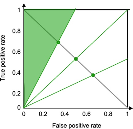
The same relations
are expressed on the new ROC curve below, now with TP rate on Y axis and FP
rate on X axis. The A and B at prevalence 33%, 50%, and 67% are represented as green
circles on the intersection between A=OR*B and A=-B+1.
Remembering from the
previous section that restricting the threshold while keeping Prevalence
constant steepens the slope of <![if !msEquation]><![if !vml]>![]() <![endif]><![endif]>,
this can be represented on the graph as a TP/FP region of possible slopes,
defined as the area covered by this equation with slope varying from OR to
∞:
<![endif]><![endif]>,
this can be represented on the graph as a TP/FP region of possible slopes,
defined as the area covered by this equation with slope varying from OR to
∞:
|
<![if !vml]> |
<![if !vml]> |
<![if !vml]> |
|
TP/FP region of possible
slopes at prevalence 67% i.e. OR=2 |
TP/FP region of possible
slopes at prevalence 50% i.e. OR=1 |
TP/FP region of possible
slopes at prevalence 33% i.e. OR=1/2 |
 <![endif]>
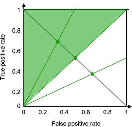 <![endif]>
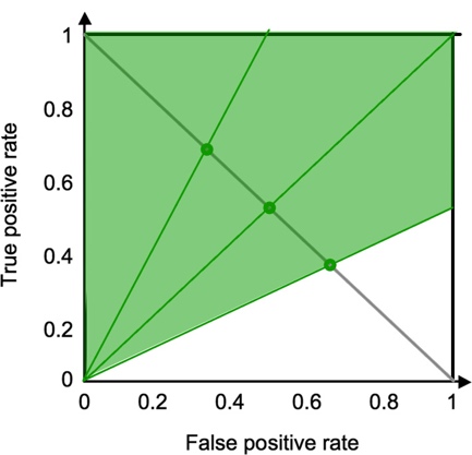 <![endif]>
What this region of possible
slopes does not represent is exactly where TP and FP are. Is it possible to
figure out the exact TP & FP other than at the most lenient threshold (the green
circles)? Yes, and this is where plots on the other ROC curve definition fits
in.
Overlay the Sens/Spec curve on TP/FP
curve
On the TP/FP ROC
curve, Y axis = TP = A; X axis = FP = B.
On the Sens/Spec ROC
curve, Y axis = Sensitivity = A/(A+C); X axis = (1-Specificity) =
B/(B+D). In other words, Y axis = Sensitivity = A/Prevalence; X axis =
B/(1-Prevalence).
Therefore, in reverse,
the Y value of the TP/FP ROC curve is the Y value of the Sens/Spec ROC curve
times Prevalence; the X value of the TP/FP ROC curve is the X value of
the Sens/Spec ROC curve times (1-Prevalence). On the coordinates, this appears
as vertical and horizontal axial compressions: both Y and X values shrink
because they are multiplied with a positive value ≤1.
At the top right
corner of the Sens/Spec ROC curve, i.e. where the threshold is infinitely
lenient, the compressed coordinate matches the green dots. At the bottom left
of the Sens/Spec ROC curve, i.e. where the threshold is infinitely strict, the
compressed coordinate matches the origin (0, 0). Putting these concepts
together, below are the same ROC curve at Prevalence of 76%, 50%, and 33%:
<![if !vml]>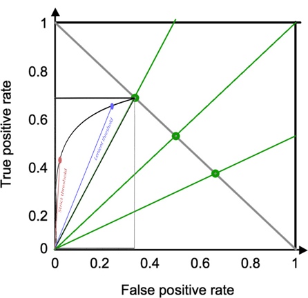 <![endif]> <![if !vml]>
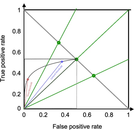 <![endif]><![if !vml]>
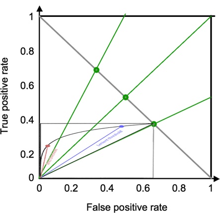 <![endif]>
Note that the red and
blue dots each represent the same test result thresholds. One can appreciate how
differently the dots are located depending on prevalence, i.e. depending on
where along the gray line to fit the top right corner of the curve.
One may also
appreciate how the optimal test threshold depends on prevalence. The top left
corner at (X, Y) = (FP, TP) = (0, 1) is always the ideal test result, which is
simply not achievable with disease prevalence <1 and overlapping result histograms.
However, the optimal point can still be defined as the point on the ROC curve
that is closest to (X, Y) = (0, 1). The precise derivation of optimal point is beyond
the scope as it requires knowing the specific test result histograms.
Conceptually, one can imagine an expanding circle centered on (X, Y) = (0, 1),
with the point that it touches first on the black curve being closest to (0, 1)
and hence optimal. That point is much closer to the blue dot when Prevalence
= 67% than when Prevalence = 50%, and closer to the red circle
when Prevalence = 33%.
Fitting in the region of utility
in this coordinate
On the Sens/Spec ROC,
<![if !msEquation]><![if !vml]>![]() <![endif]><![endif]>
<![endif]><![endif]>
<![if !msEquation]><![if !vml]>![]() <![endif]><![endif]>
<![endif]><![endif]>
To transform this relationship to the TP/FP coordinate, take the axis compression into account:
<![if !msEquation]><![if !vml]>![]() <![endif]><![endif]>
<![endif]><![endif]>
<![if !msEquation]><![if !vml]>![]() <![endif]><![endif]>
<![endif]><![endif]>
Thus, the area
left of the slope <![if !msEquation]><![if !vml]>![]() <![endif]><![endif]> is defined as the TP/FP region of
utility. Minimal possible PPV is = Prevalence @ most lenient
threshold maximal
possible PPV is 1 @ strictest threshold, rendering the minimal possible slope
for a given Prevalence (ignoring the PPVmingoal) to be
the same as the green lines. In other word, if one arbitrarily selects a
minimal goal PPV that is smaller than the Prevalence in one’s target
population, one might as well not set a goal, and feel free to select the
globally optimal point on the ROC.
<![endif]><![endif]> is defined as the TP/FP region of
utility. Minimal possible PPV is = Prevalence @ most lenient
threshold maximal
possible PPV is 1 @ strictest threshold, rendering the minimal possible slope
for a given Prevalence (ignoring the PPVmingoal) to be
the same as the green lines. In other word, if one arbitrarily selects a
minimal goal PPV that is smaller than the Prevalence in one’s target
population, one might as well not set a goal, and feel free to select the
globally optimal point on the ROC.
When drawing the slope corresponding to minimal goal PPV, one can appreciate that having a high Prevalence leaves a greater portion of the ROC curve on the left side of the minimal goal PPV slope. Thus, it allows a greater range of thresholds, including the more lenient ones. This is the same conclusion as in the experiment on the Sens/Spec ROC curve.
<![if !vml]>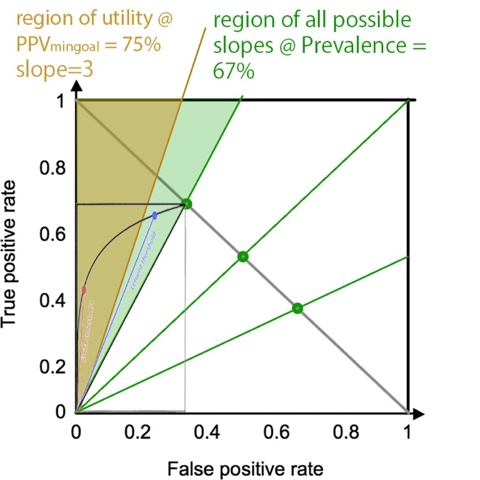 <![endif]><![if !vml]>
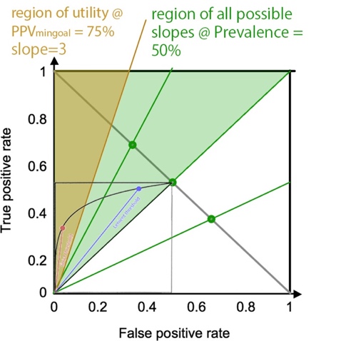 <![endif]> <![if !vml]>
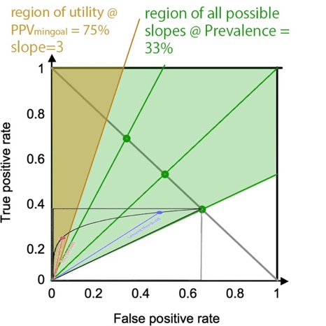 <![endif]>
Question when should (Sensitivity,
Specificity) vs (TP, 1-FP) be optimized?
Picking a PPV based on pre-test OR
and desired post-test OR
When one wants to
raise the post-test disease odds ratio to a certain percentage provided a known
disease prevalence, one must satisfy LR+ via this formula:
Post-test OR+
= Pre-test OR * LR+
Post-test OR-
= Pre-test OR * LR-
Derivation:
For OR+:
<![if !supportLists]>-
<![endif]>Chance of
testing (+) in a randomly picked person = chance of true (+) + chance of false
(+) = Odds numerator * Sens + Odds denominator * (1-Spec)
<![if !supportLists]>-
<![endif]>Given a
(+) test, Post-test Odds of having disease / no disease = <![if !msEquation]><![if !vml]>![]() <![endif]><![endif]>
<![endif]><![endif]>
For OR-:
<![if !supportLists]>-
<![endif]>Chance of
testing (-) in a randomly picked person = chance of false (-) + chance of true
(-) = Odds numerator *(1-Sens) + Odds denominator * Spec
<![if !supportLists]>-
<![endif]>Given a
(-) test, Post-test Odds of having disease / no disease = <![if !msEquation]><![if !vml]>![]() <![endif]><![endif]>
<![endif]><![endif]>
Given the slope
formula for the TP/FP ROC curve,<![if !msEquation]><![if !vml]>![]() <![endif]><![endif]>
<![endif]><![endif]>
<![if !msEquation]><![if !vml]>![]() <![endif]><![endif]>
<![endif]><![endif]>
<![if !vml]>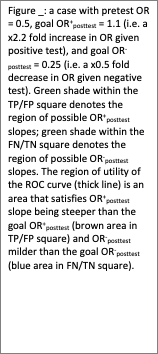 <![endif]><![if !vml]>
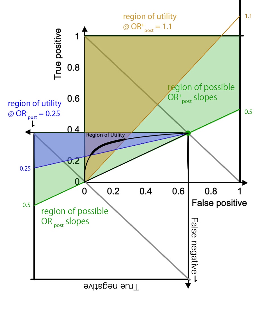 <![endif]>
Application
<![if !supportLists]>1.
<![endif]>Draw a square
coordinate with origin (X=0, Y=0) at bottom left and span of up to X=1 (going
right) and Y=1 (going up).
<![if !supportLists]>2.
<![endif]>Obtain the
disease prevalence of your population. Calculate ORpretest = Prevalence/(1-Prevalence).
Draw a line from the origin to (X=1, Y=ORpretest).
<![if !supportLists]>3.
<![endif]>Draw a
line from the origin to (X=1, Y=OR+posttest goal). The slope
will be OR+posttest = <![if !msEquation]><![if !vml]>![]() <![endif]><![endif]> = LR+
* ORpretest.
<![endif]><![endif]> = LR+
* ORpretest.
<![if !supportLists]>4.
<![endif]>Draw a
line from (X=0, Y=1) to (X=1, Y=0). The intersection between this line and the
line from Step 1 is where the top right corner of the Sens/Spec ROC curve will
fit.
<![if !supportLists]>5.
<![endif]>Fit the
Sens/Spec ROC curve. Place the top right corner at the intersection on Step 3; place
the bottom left corner at the origin.
<![if !supportLists]>6.
<![endif]>Look for
the intersection between the line from Step 2 and the fitted ROC curve. Is
there any portion of the ROC curve inside the region of utility left of/above
the Step 2 line? If not, this test is not suitable. Either lower the OR+posttest
goal or pick another test with a better Sens/Spec ROC characteristic at the
strict end of its threshold. If yes, continue.
<![if !supportLists]>7.
<![endif]>Draw the
second square coordinate, with origin at top right overlapping the ROC curve’s
top right point, and span of up to X=1 (going left) and Y=1 (going down).
<![if !supportLists]>8.
<![endif]>Extend the
ORpretest slope to bottom left to fill the second square coordinate.
This line should hit the second (upside-down) coordinate’s left edge at (X=1,
Y=ORpretest).
<![if !supportLists]>9.
<![endif]>Draw a
line from the origin of the second (upside-down) coordinate to (X=1, Y=OR-posttest).
The slope will be OR-posttest = <![if !msEquation]><![if !vml]>![]() <![endif]><![endif]>=LR-*ORpretest.
<![endif]><![endif]>=LR-*ORpretest.
<![if !supportLists]>10.
<![endif]>Look for the intersection between the line from
Step 9 and the fitted ROC curve. Is there any portion of the ROC curve inside
the region of utility to the left of/above the Step 9 line? If not, this
test is not suitable. Either loosen (i.e. larger # = closer to ORpretest
= milder decrease from ORpretest) the OR-posttest
goal or pick another test with a better Sens/Spec ROC characteristic at the
lenient end of its threshold. If yes, continue.
<![if !supportLists]>11.
<![endif]>Look for the overlapping regions of utility
defined by Steps 6 and 10. Pick a threshold within this region that maximizes
Sens and Spec.
LR+ and LR-
of sequential tests can be multiplied on top of pretest odds, such that each subsequent
test drives the OR+posttest farther up and OR-posttest
farther down:
<![if !msEquation]><![if !vml]>![]() <![endif]><![endif]>
<![endif]><![endif]>
<![if !msEquation]><![if !vml]>![]() <![endif]><![endif]>
<![endif]><![endif]>
Remember to set ORpretest
of (n+1)-th test to the ORposttest of n-th test. More on this method:
(1)
Precision-Recall curve 20200210
Precision and Recall
are defined below, with their respective extrema.
|
|
Strict threshold |
Lenient threshold |
|
X-axis = Recall =
Sensitivity = <![if !msEquation]><![if !vml]> |
0 ≤ low |
high ≤ 1 |
|
Y-axis = Precision =
PPV = <![if !msEquation]><![if !vml]> |
high ≤ 1 |
Prevalence ≤ low |
|
Slope through origin
= <![if !msEquation]><![if !vml]> |
high ≤ <![if !msEquation]><![if !vml]> |
high ≤ Prevalence |
An indiscriminative (“no
skill”) test will have X ranging from 1 to 0 as threshold becomes stricter, and
Y = Prevalence.
<![if !vml]> <![endif]>The
following equation describes Y as a function of X:
<![endif]>The
following equation describes Y as a function of X:
<![if !msEquation]><![if !vml]> <![endif]><![endif]>
On the surface, X <span lang=ZH-TW style='font-family:"PMingLiU",serif; mso-ascii-font-family:Calibri;mso-ascii-theme-font:minor-latin;mso-fareast-theme-font: minor-fareast;mso-hansi-font-family:Calibri;mso-hansi-theme-font:minor-latin'>→</span><span lang=ZH-TW> </span>0 may seem to result in Y <span lang=ZH-TW style='font-family:"PMingLiU",serif;mso-ascii-font-family: Calibri;mso-ascii-theme-font:minor-latin;mso-fareast-theme-font:minor-fareast; mso-hansi-font-family:Calibri;mso-hansi-theme-font:minor-latin'>→</span> 0. However, the reason that Y = PPV<span lang=ZH-TW style='font-family:"PMingLiU",serif; mso-ascii-font-family:Calibri;mso-ascii-theme-font:minor-latin;mso-fareast-theme-font: minor-fareast;mso-hansi-font-family:Calibri;mso-hansi-theme-font:minor-latin'>→</span><span lang=ZH-TW> </span>1 as X=Sensitivity <span lang=ZH-TW style='font-family: "PMingLiU",serif;mso-ascii-font-family:Calibri;mso-ascii-theme-font:minor-latin; mso-fareast-theme-font:minor-fareast;mso-hansi-font-family:Calibri;mso-hansi-theme-font: minor-latin'>→</span> 0 which happens with a strict threshold is that Specificity is not totally independent of Sensitivity in any test with overlapping values for diseased vs healthy population, therefore LR+ <span lang=ZH-TW style='font-family:"PMingLiU",serif;mso-ascii-font-family:Calibri; mso-ascii-theme-font:minor-latin;mso-fareast-theme-font:minor-fareast; mso-hansi-font-family:Calibri;mso-hansi-theme-font:minor-latin'>→</span><span lang=ZH-TW> </span><span lang=ZH-TW style='font-family:"PMingLiU",serif; mso-ascii-font-family:Calibri;mso-ascii-theme-font:minor-latin;mso-fareast-theme-font: minor-fareast;mso-hansi-font-family:Calibri;mso-hansi-theme-font:minor-latin'>∞</span><span lang=ZH-TW> </span>while 1/OR stays constant. This trend of LR+ is also demonstrated on the steepening slope of Sens/Spec curve through origin.
The precision-recall curve is another way to visualize the PPV-to-Sensitivity tradeoff when setting a PPVmingoal. Namely, the region of utility is above the horizontal line defined by Y=PPVmingoal, restricting X to its lower end. Just like in the TP/FP ROC discussion, a PPVmingoal below the Prevalence of one’s target population is nonsensical because all (X,Y) are necessarily above Y=Prevalence. One should then feel free to select the globally optimal point closest to (X,Y) = (1,1).
Drop in Prevalence depresses Y more at the higher end
of X, since the increase in the term <![if !msEquation]><![if !vml]>![]() <![endif]><![endif]> affects PPV more when <![if !msEquation]><![if !vml]>
<![endif]><![endif]> affects PPV more when <![if !msEquation]><![if !vml]>![]() <![endif]><![endif]> is small.
<![endif]><![endif]> is small.
<![if !msEquation]><![if !vml]>![]() <![endif]><![endif]>
<![endif]><![endif]>
«««< Updated upstream
1-Y is not directly proportional to 1-Prev.